Posted on

Use Python to get more than 0.75 accuracy in Titanic problem by Kaggle

Ship_image
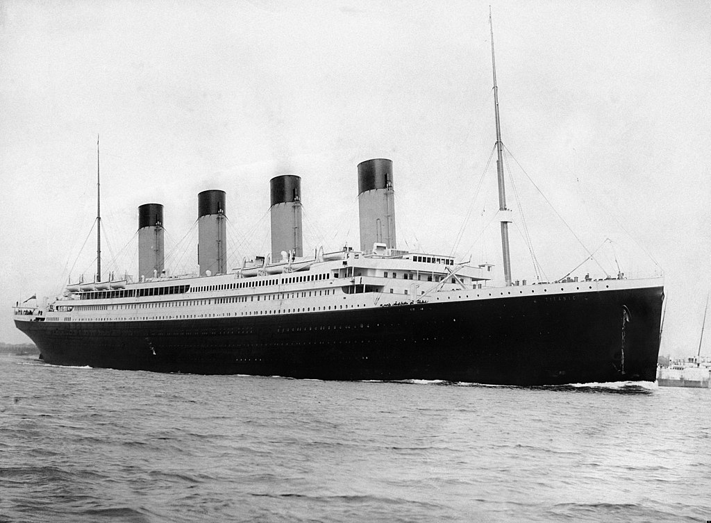
The sinking of the RMS Titanic is one of the most infamous shipwrecks in history. On April 15, 1912, during her maiden voyage, the Titanic sank after colliding with an iceberg, killing 1502 out of 2224 passengers and crew. This sensational tragedy shocked the international community and led to better safety regulations for ships. One of the reasons that the shipwreck led to such loss of life was that there were not enough lifeboats for the passengers and crew. Although there was some element of luck involved in surviving the sinking, some groups of people were more likely to survive than others, such as women, children, and the upper-class.

The problem statement was to complete the analysis of what sorts of people were likely to survive and apply the machine learning tools to predict which passengers survived the tragedy. The Kaggle Titanic problem page can be found here. The full solution in python can be found here on github. The data in the problem is given in two CSV files, test.csv and train.csv. The variable used in the data and their description are as follows

Variable Name Definition
survival If an individual survived the tragedy or not
pclass Ticket class
Name Name of the individual
sex Sex
Age Age in years
sibsp # of siblings/spouses aboard the Titanic
parch # of parents/children aboard the Titanic
ticket Ticket Number
fare Passenger fare
cabin Cabin Number
embarked Port of Embarkation

The target variable here is Survived which takes the value 0 or 1. Since the target value takes the binary values we can say that the this is an example of classification problem. We have to train the model using train.csv and predict the outcomes using test.csv and submit the predictions on kaggle. At first we will read the data from CSV file using the pandas library in python, for that we have to import pandas library. The data is loaded in pandas dataframe format. We can see how the data looks like using dataframe.head() command. We can also see the columns using dataframe.columns command. We can check the number of rows and columns of the dataframe using the dataframe.shape command.

import pandas as pd
dataframe=pd.read_csv('train.csv')
print(dataframe.head(10))
print(dataframe.columns)
print(dataframe.shape)

The ‘Name’ variable present here contains the full name of the person. In this format the ‘Name’ variable is not useful for us as almost all the entries here will be unique and that would not help in our prediction. We can make this useful by trimming and partitioning the string to get the title and first name of the individual.

dataframe['Name']=dataframe['Name'].str.partition(',')[2]
dataframe['Name']=dataframe['Name'].str.partition(',')[0]

We can check the values taken by a variable by values_count() function. We can also check whether a variable contains NaN(Not a Number) values or not. After checking value_counts for age variable we found out that the age variable contained NaN values. We can wither drop the NaN values using dropna() function or we can impute the values. In this example we will impute the missing values using MICE(Multiple Imputation by Chained Equations). To use MICE function we have to import a python library called ‘fancyimpute’. Mice uses the other variables to impute the missing values and iterate it till the value converges such that our imputed value balances the bias and variance of that variable.

print(dataframe['Age'].value_counts(dropna=False)
from fancyimpute import MICE
solver=MICE()
Imputed_dataframe=solver.complete(dataframe.values)

Since this is a classification problem we can solve it by methods such as Logistic Regression, Decision Tree, Random Forest etc. Here we will use Random Forest to solve this problem. Variables present here are categorical and continuous. Some of the categorical variables are in the string format. So we have to first change that in the integer categorical format so that we can feed the data directly for our model to learn. We can use factorize function from pandas library to do this.

cols=['Name','Ticket','Pclass','Fare','Embarked','Cabin']
for x in cols:
    a=pd.factorize(dataframe[x])
    dataframe[x]=a[0]

We can create an addition variable named ‘family_size’ using the variables ‘parch’ and ‘sibsp’. Now our data is ready and we can train our model using the data. We will first divide the data into target variables and and features as Y and X. We will train the model using X and Y.

dataframe['family_size']=dataframe['SibSp'] + dataframe['Parch'] + 1
y=dataframe[['Survived']].values
x=dataframe.values
import numpy as np
x=np.delete(dataframe,0,axis=1)
model=RandomForestClassifier(n_estimators=100,criterion='gini',max_depth=10,min_samples_split=10)
model=model.fit(x,y)

Now our model has been trained. We can use this model to predict whether a person survived the tragedy or not. Now we will read the test.csv file and use the variables present as test features for prediction.

test=pd.read_csv('test.csv')
test['Name']=test['Name'].str.partition(',')[2]
test['Name']=test['Name'].str.partition('.')[0]
cols=['Name','Ticket','Pclass','Fare','Embarked','Cabin']
for x in cols:
    a=pd.factorize(test[x])
    test[x]=a[0]
test_features=test.values
my_prediction = model.predict(test_features)

Now we have our predictions in ‘my_prediction’ variable. Now we are ready to submit the solution to kaggle. For kaggle submission a specific format is given for problems. We will write our solution in a CSV file in suitable format which we can submit at kaggle.

PassengerId =np.array(test["PassengerId"]).astype(int)
my_solution = pd.DataFrame(my_prediction, PassengerId, columns = ["Survived"])
my_solution.to_csv("my_solution.csv", index_label = ["PassengerId"])

Now we have our solution in a CSV file ‘my_solution.csv’. We can submit this file on to kaggle submission page and check our accuracy.


Posted on

Node-RED for Internet of Things

Node RED

Node-RED is a programming tool developed by IBM for wiring together hardware devices, APIs and online services in new and interesting ways.

It is built on Node.js, taking full advantage of its event-driven, non-blocking model. This makes it ideal to run at the edge of the network on low-cost hardware such as the Raspberry Pi as well as in the cloud.

It provides a browser-based editor that makes it easy to wire together flows using the wide range of nodes in the palette that can be deployed to its runtime in a single-click.
Features

  • Browser-based flow editing
  • Built on Node.js
  • Social Development

Node-RED Comes along with the Bluemix IOT Starter Application. Adding IoT Foundation Service with Bluemix allows to use Node-RED. You can use the incoming and outgoing MQTT nodes in your flows. Most of them use Node-RED to define flows where either incoming sensor data from ‘things’ is handled, e.g. stored in databases, or where commands are sent to devices.

GitHub Link: https://github.com/node-red/node-red

Posted on

Google announced a private beta of their Google IoT Core platform

In a recent blog post, Google announced a private beta of their Google IoT Core platform. Cloud IoT Core makes it easy to securely connect your globally distributed devices to GCP, centrally manage them and build rich applications by integrating with their data analytics services. Furthermore, all data ingestion, scalability, availability and performance needs are automatically managed for you in GCP style.
When used as part of a broader Google Cloud IoT solution, Cloud IoT Core gives you access to new operational insights that can help your business react to and optimize for change in real time. This advantage has value across multiple industries; for example:


  • Utilities can monitor, analyze and predict consumer energy usage in real time
  • Transportation and logistics firms can proactively stage the right vehicles/vessels/aircraft in the right places at the right times
  • Oil, gas and manufacturing companies can enable intelligent scheduling of equipment maintenance to maximize production and minimize downtime

So, why is this the right time for Cloud IoT Core?

About all the things

Many enterprises that rely on industrial devices such as sensors, conveyor belts, farming equipment, medical equipment and pumps — particularly, globally distributed ones — are struggling to monitor and manage those devices for several reasons:

  • Operational cost and complexity: The overhead of managing the deployment, maintenance and upgrades for exponentially increasing devices is stifling. And even with a custom solution in place, the resource investments required for necessary IT infrastructure are significant.
  • Patchwork security: Ensuring world-class, end-to-end security for globally distributed devices is out of reach — or at least not a core competency — for most organizations.
  • Data fragmentation: Despite the fact that machine-generated data is now an important data source for making good business decisions, the massive amount of data generated by these devices is often stored in silos with a short expiration date, and hence never reaches downstream analytic systems (nor decision makers).

Cloud IoT Core is designed to help resolve these problems by removing risk, complexity and data silos from the device monitoring and management process. Instead, it offers you the ability to more securely connect and manage all your devices as a single global system. Through a single pane of glass you can ingest data generated by all those devices into a responsive data pipeline — and, when combined with other Cloud IoT services, analyze and react to that data in real time.

GCP

Key features and benefits

Several key Cloud IoT Core features help you meet these goals, including:

  • Fast and easy setup and management: Cloud IoT Core lets you connect up to millions of globally dispersed devices into a single system with smooth and even data ingestion ensured under any condition. Devices are registered to your service quickly and easily via the industry-standard MQTT protocol. For Android Things-based devices, firmware updates can be automatic.
  • Security out-of-the-box: Secure all device data via industry-standard security protocols. (Combine Cloud IoT Core with Android Things for device operating-system security, as well.) Apply Google Cloud IAM roles to devices to control user access in a fine-grained way.
  • Native integration with analytic services: Ingest all your IoT data so you can manage it as a single system and then easily connect it to our native analytic services (including Google Cloud Dataflow, Google BigQuery and Google Cloud Machine Learning Engine) and partner BI solutions (such as Looker, Qlik, Tableau and Zoomdata). Pinpoint potential problems and uncover solutions using interactive data visualizations, or build rich machine-learning models that reflect how your business works.
  • Auto-managed infrastructure: All this in the form of a fully-managed, pay-as-you-go GCP service, with no infrastructure for you to deploy, scale or manage.

iot-core-2


Posted on

Why MEAN is better than LAMP ?


Developing a Web-driven application (either mobile or browser-based) typically requires the provisioning of some server-side infrastructure as well as the development of some code to run on it. Such code will often consume APIs. But occasionally, it provide them as well. For many years, the go-to infrastructure in such situations was affectionately referred to as the LAMP stack and it primarily involved Linux, Apache, MySQL and PHP, Perl or Python. But, thanks in part to Javascript’s applicability to both client and server-side scripting, there’s an another stack that’s now widely considered as an alternative to LAMP; the MEAN stack.


What’s LAMP?

linux-2025536_640

Linux, Apache, MySQL and PHP. The holy grail of web development for at least as long as I can remember. This stack represents the foundation of the web.

While its age may be showing, its maturity is strong. The LAMP stack can be altered to replace MySQL with MongoDB, and PHP with Python. The acronym defines a low level configuration for web applications.

What’s MEAN?

Meanstack-624x250


MongoDB, ExpressJS, AngularJS and Node.js makes up the MEAN stack. A powerful JavaScript driven stack with diverse capabilities.

Comparatively to LAMP, the database layer is replaced completely with JSON storage using MongoDB. JSON is the native data language of JavaScript. While relatively young, the framework has a growing number of supporters.

This stack is basically a JavaScript lover’s dream.

Now we will look at points , why MEAN is better.


Node.js is superfast


Apache was great, but these days, Node.js is often flat-out faster. A number of benchmarks show that Node.js offers better performance, while doing much more. Perhaps it’s the age of the code. Perhaps the Node.js event-driven architecture is quicker. It doesn’t matter. These days, especially among impatient mobile device users, shaving even milliseconds off your app’s performance is important and Node.js can do that, while offering a Turing-complete mechanism for reprogramming it.


MongoDB is built for the cloud


If your Web app plans include making good on the pennies-per-CPU promise of the cloud, the MEAN stack offers a compelling database layer in MongoDB. This modern database comes equipped with automatic sharding and full cluster support, right out of the box. Plug in MongoDB and it spreads across your cluster of servers to offer failover support and automatic replication. Given the ease with which apps can be developed, tested, and hosted in the cloud, there’s little reason not to consider MongoDB for your next project.


MySQL’s structure is confining (and overrated)


Anyone who has developed or maintained a LAMP-based app for any amount of time knows that MySQL’s strength as a relational database can feel a bit imprisoning at times. Like all relational databases, MySQL forces you to push your data into tables. This isn’t a problem if every single entry fits into exactly the same format, but how often is the world that generous? What if two people share the same address but not the same account? What if you want to have three lines to the address instead of two? Who hasn’t tried to fix a relational database by shoehorning too much data into a single column? Or else you end up adding yet another column, and the table grows unbounded.

MongoDB, on the other hand, offers a document structure that is far more flexible. Want to add a new bit of personal information to your user profiles? Simply add the field to your form, roll it up with the rest of the data in a JSON document, and shove it into your MongoDB collection. This is great for projects in flux and for dealing with data that may ultimately prove tricky to constrain in table form.


Angular is a Plus


It’s not exactly fair to compare the “A” in “MEAN” with anything in the LAMP stack because LAMP doesn’t include an analog. If you want to do anything on the client side, you’re on your own. Sure, there are plenty of good PHP-based frameworks that work with MySQL, but each is a bit different and moving in its Angular_full_color_logo.svgown direction. AngularJS has been developed as well as maintained by dedicated Google engineers. This means that there is a huge community out there for you to learn from. Apart from that, there are engineers that can help you tackle any challenges you face on the way. It also means that clients get what they want. Most frameworks require programmers to splitting the app into multiple MVC components. After that, the programmer has to write a code to put them together again. AngularJS, however, strings it together automatically. That saves you time, and reduces the app’s time-to-market.


AngularJS is more intuitive as it makes use of HTML as a declarative language. Moreover, it is less brittle for reorganizing. AngularJS is a comprehensive solution for rapid front-end development. It does not need any other plugins or frameworks. Moreover, there are a range of other features that include Restful actions, data building, dependency injection, enterprise-level testing, etc. AngularJS is unit testing ready, and that is one of its most compelling advantages.


Node.js simplifies the server layer


Node.js_logo

Navigating the various layers of the LAMP stack can be a difficult dance of many hats, one that has you shuffling through various config files with differing syntax. MEAN simplifies this through use of Node.js.

Want to change how your app routes requests? Sprinkle in some JavaScript and let Node.js do the rest. Want to change the logic used to answer queries? Use JavaScript there as well. If you want to rewrite URLs or construct an odd mapping, it’s also in JavaScript. The MEAN stack’s reliance on Node.js put this kind of pipework all in one place, all in one language, all in one pile of logic. You don’t need to reread the man pages for PHP, Apache, and whatever else you add to the stack. While the LAMP generation has different config files for everything, Node.js avoids that issue altogether. Having everything in one layer means less confusion and less chance of strange bugs created by weird interactions between multiple layers.


JSON everywhere


AngularJS and MongoDB both speak JSON, as do Node.js and Express.js. The data flows neatly among all the layers without rewriting or reformatting. MySQL’s native format for answering queries is, well, all its own. Yes, PHP already has the code to import MySQL data and make it easy to process in PHP, but that doesn’t help the client layer. This may be a bit minor to seasoned LAMP veterans because there are so many well-tested libraries that convert the data easily, but it all seems a bit inefficient and confusing. MEAN uses the same JSON format for data everywhere, which makes it simpler and saves time reformatting as it passes through each layer. Plus, JSON’s ubiquity through the MEAN stack makes working with external APIs that much easier: GET, manipulate, present, POST, and store all with one format.


Its your choice


Of course, if you’re really picky, there’s no reason why you can’t mix it up a bit. Plenty of developers use MongoDB with Apache and PHP, and others prefer to use MySQL with Node.js. AngularJS works quite well with any server, even one running PHP to deliver data from MySQL. You don’t have to be a slave to the acronyms.

programming-1873854_640

This post is inspired from another blog written on this topic


Posted on

Use Python for Data Cleaning and Analyzing nicotine dependence

doc(1)

The objective of the project was to study Nicotine Dependence. Nicotine Dependence is an addiction to tobacco products caused by the drug nicotine. At first association between smoking behaviour and Nicotine Dependence was explored. Social behaviour and depression history were then analyzed as explanatory variables. A study at Universiti Teknologi MARA Malaysia concluded that among smokers 5% have high nicotine dependence whereas 18% have moderate nicotine dependence. Another study by the Durham University , UK found that life events and stressful experiences are associated with nicotine dependence.

The data was taken from a survey conducted by National Epidemiologic Survey on Alcohol and Related Conditions (NESARC). Earlier National Institute on Alcohol Abuse and Alcoholism have performed landmark study on Alcohol Abuse and Alcohol Dependence using the NESARC dataset.  The dataset is a representative sample of United States adult population aged over 18. Initially the data consisted of over 43000 data points.

The data was in Comma Separated Value(CSV) format. The variables used for the regression model were.

Variable Name Description
CHECK321 the cigarette smoking status of the individual
S3AQ3B1 the usual frequency when the individual smoked cigarettes
S3AQ3C1 the usual quantity when the individual smoked
TAB12MDX the dependent variable which represented if the respondent had a nicotine dependence in the last 12 months

The dataset contained various missing values. Python was the language used for the data cleaning and analysis purpose. At first using the pandas library in python the dataset was loaded. After loading the the data missing values of the CHECK321 variable were checked. The unknown values of the CHECK321 suggested that the cigarette smoking status of an individual is unknown and so the analysis can not be done for that individual. Hence the data points containing missing values of CHECK321 were deleted. After deleting the missing values we were left with 18000 data points. The target variable TAB12MDX took only two values ‘0’ and ‘1’. ‘1’ denoting the individual is nicotine dependent and ‘0’ denoting that the individual is not nicotine dependent.

telepain

For analysis of the data we split the data and into training and testing set. Training data was used to train our model. Since the target variable is binary we decided to use logistic regression for training the model. For splitting the data we used a python library Scikit Learn also popular as sklearn. The training test split ratio was 80:20. The cleaned data was fed to the model and the model was trained. After training the model we tested the model with the test data we had split earlier. We saw that for 58% of the times our model has correctly predicted whether a person is nicotine dependent.

As the study by the Durham University , UK found that life events and stressful experiences are also associated with nicotine dependence. We decided to introduce two new variables MAJORDEPLIFE and SOCPDLIFE to make our model more accurate.


Variable Name Description
MAJORDEPLIFE If the individual suffered depression or not
SOCPDLIFE If the individual has socio-phobia or not

We again split our data into training and testing sets. The model was trained with the testing set now with two new variables. Now with the introduction of two new variables associated with the life events and stressful experience the accuracy of our model increased to 65%. For 65% of the times we predicted correctly whether a person is nicotine dependent or not by seeing is smoking behaviour and social life.
Research concludes that individual who smoke more heavily than those who don’t are more prone to be Nicotine Dependent. Individuals who have a history of Depression or are Socio-phobic are also more prone to be Nicotine Dependent than those without.Our results seems consistent with the previous findings.